Tumor growth under drug treatment#

This example presents a simple model of tumor growth coupled with the administration of an antitumor drug. The original research and the modeling methodology are detailed in Drexler et al. (2020).

Background#

The original paper’s experiments investigate the response of a murine breast cancer model to pegylated liposomal doxorubicin (PLD or Doxil) over a long time frame (approximately 80 to 250 days). The authors proposed a system of ordinary differential equations (ODEs) to describe the dynamics of tumor cells, necrotic cells, and drug levels in both the tumor tissue (central compartment) and peripheral organs (peripheral compartment). The drug treatment is modeled by instant changes to the drug levels in the central compartment at specific time points, corresponding to the actual injections administered in the in vivo experiment.

The equations of the mathematical model are as follows.

\[\begin{split}\begin{align*} \dot{x}_1 &= (a - n) x_1 - b \frac{x_1 x_3}{ED_{50} + x_3} \\ \dot{x}_2 &= n x_1 + b \frac{x_1 x_3}{ED_{50} + x_3} - w x_2 \\ \dot{x}_3 &= -(c + k_1) x_3 + k_2 x_4 - b_k \frac{x_1 x_3}{ED_{50} + x_3} \\ \dot{x}_4 &= k_1 x_3 - k_2 x_4 \end{align*}\end{split}\]

Here, the state variables \(x_1\) and \(x_2\) represent the tumor tissue volume and the necrotic tissue volume (in mm³ ). Variables \(x_3\) and \(x_4\) correspond to the drug levels (in mg/kg) in the central and peripheral compartments, respectively.

The model incorporates the following dynamics:

Tumor cells proliferate at a known duplication rate (\(a\)).
Tumor cells undergo spontaneous necrosis at a rate (\(n\)) independent of the drug level.
Tumor cells convert into necrotic cells based on the drug level (\(x_3\)) and the drug’s specific properties (explained below).
Necrotic cells are removed from the tissue (washout) at a known rate (\(w\)).
The drug is administered instantaneously, resulting in an immediate change to the level of \(x_3\).
The drug is distributed between the two compartments, with transport governed by rates \(k_1\) (central to peripheral) and \(k_2\) (peripheral to central).

Fig. 1 shows a representative in vivo experimental result. The red dots represent the measured data series obtained by regularly monitoring the size (volume) of the tumor tissue implanted in the mouse.

By appropriately selecting the model parameters (fitting the model) and accounting for the treatment effects, this ODE model approximates the observed dynamics in reality: the rapidly growing tumor without treatment, followed by the volume decrease due to the treatment, which is explained by the death and clearance of the tumor tissue cells. After treatment, the drug is continuously cleared, thus its effect diminishes, leading to tumor regrowth.

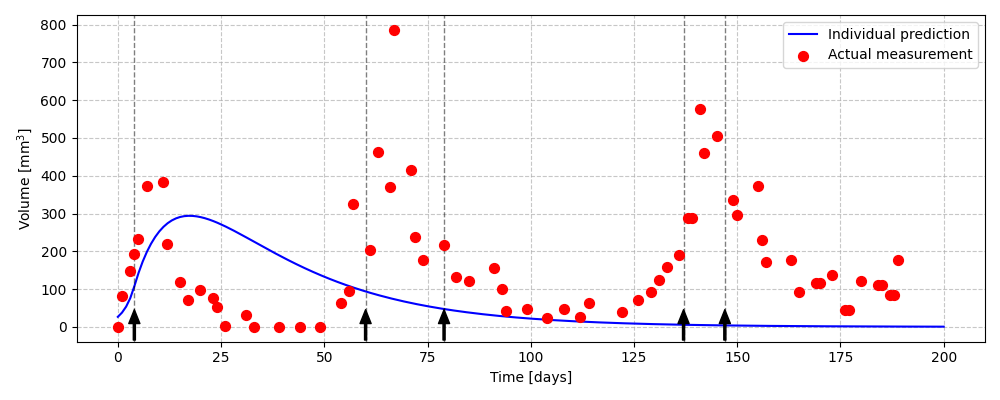
../../_images/drug_treatment_fig1.png — Fig. 1 Actual tumor volumes measured during an experiment (red dots) and the simulated volumes obtained after fitting the model (blue line). The times of drug treatments are indicated by black arrows. (Re-plotted from data in Drexler et al. (2020).)#

LattiCS implementation#

We will implement the experiment in LattiCS in two ways. Initially, a homogeneous simulation space (mirroring the ODE model) will serve as a surrogate model for parameter estimation. This will be followed by a two-dimensional simulation space to specifically model a slice of a spatial tumor. When LattiCS uses a homogeneous simulation space, it disregards all spatial properties of agents and substrates, significantly accelerating the simulation. This simplifies the model to only tracking cell counts and average substrate concentrations, similar to an ODE model. However, unlike a deterministic ODE model, the agent-based approach still uses stochastic update steps, meaning simulation results may differ due to random effects (e.g., in cell division or cell death).

Following the selection of the simulation space, the model setup will proceed in two major steps: first, tuning the parameters of the drug introduced during the treatments, and subsequently, adding the agents that describe the tumor tissue cells to the model.

Initial steps#

First, we load the lattics package and create a Simulation object and a HomogeneousSpace object. We use a 1-hour time step for the agents’ simulation and a 30-second time step for the substrate (drug) simulation.

For practical reasons, ensuring compatibility with subsequent 2D slice-based simulations, the volume of the computational space is fixed at 8.4375 × 10⁶ μm³. This corresponds to a 15 μm thick slice of a 750 μm × 750 μm region, deliberately chosen to facilitate direct comparison between the initial virtual model and its future 2D cross-section. This choice of volume primarily determines the maximum cell capacity, thus influencing the simulation speed. Given the agent volumes (see below), this space will accommodate a maximum of 2500 agents, a simulation that should take no more than a few minutes on an average personal computer.

import lattics

simulation = lattics.Simulation()
space = lattics.HomogeneousSpace(
        simulation=simulation,
        dt_agent=(1, 'hour'),
        dt_substrate=(30, 'sec'),
        volume=8.4375 * 10 ** 6
        )
simulation.add_space(space)

The pharmacokinetics of the drug#

In the animal experiments, the drug is administered to the subjects as a bolus injection, which causes its concentration in the blood to instantaneously increase, followed by distribution into the tissues and subsequent elimination (or degradation) over time. The ODE model describes the drug concentration within two compartments (tumor tissue and organs). This two-compartment approach allows the model to accurately describe the measurable concentrations observed in vivo following treatment.

We now incorporate a substrate named “drug” into the simulation space. When creating the substrate, we must specify the diffusion coefficient and the decay coefficient describing spontaneous degradation of the substrate. Although diffusion will not be simulated in the homogeneous space, the diffusion coefficient can still be set here and will be required during the three-dimensional simulation. Based on literature data regarding the typical size of PLD nanoparticles (on the order of 100 nm), we will set the substrate’s diffusion coefficient to 2 × 10^-3 μm²/ms (Lee et al. (2021) and Schleyer et al. (2024)). Since the decay rate will be determined experimentally (see below), we will set it to an arbitrary placeholder value (e.g., 0.0) for now.

space.add_substrate(
        name='drug',
        diffusion_coefficient=2e-3,
        decay_coefficient=0.0
        )

In our approach, the simulation space represents the tissue surrounding the tumor, into which the drug is delivered by the blood vessels running through it. In this context, the blood vessels are considered the sources of the drug; locations where the drug concentration increases following treatment, and from which the drug subsequently diffuses to other parts of the tissue. In LattiCS, these sources can be represented by SubstrateNode objects, for which we can specify the internal drug concentration and the characteristics of transport (uptake-release) with the surrounding environment.

Since the location, shape, and distribution of the vessels cannot be accounted for in a homogeneous space, we will now create a single SubstrateNode object to represent all blood vessels within the tissue. Based on literature data, the typical blood volume fraction in tissues is 5-15% (Claridge et al. (2007) and Qi et al. (2008)). Accordingly, we will select 10% of the previously created space volume as the virtual volume for this SubstrateNode.

blood_vessels = lattics.SubstrateNode()
blood_vessels.set_attribute('volume', 8.4375 * 10 ** 5)

When modeling the transport from the node to the surrounding tissue (space), three types of parameters can be specified to describe the process. For simplicity, we model this process by assuming that the drug moves between the vessels and the tissue at a rate proportional to the concentration difference; therefore, we will only set the parameter for the passive transport rate for the SubstrateNode (the other values will remain zero).

We hypothesize that this process occurs relatively quickly, so we set the rate value to a high value (10^-3 1/ms), and the initial drug concentration to zero, which will increase as a result of the treatments.

blood_vessel_transport_info = lattics.SubstrateInfo(
        type='flux',
        concentration=0.0,
        passive_rate=1e-3
        )
blood_vessels.get_attribute('substrate_info')['drug'] = blood_vessel_transport_info
space._substrates['drug'].add_static_substrate_node(blood_vessels)

To account for the organs acting as a drug reservoir (“buffering effect”) the ODE model introduces a second compartment. We model this using a second SubstrateNode object, where the initial concentration is also zero, and which changes due to bi-directional transfer with the simulation space. For simplicity, we set its virtual volume to be equal to that of the original simulation space (however, this has no direct role, as the same dynamic can be achieved with a node of different virtual volume by appropriately choosing the transport rate constants due to the form of the transport equations). The release_rate and uptake_rate map directly to the ODE model’s \(k_1\) and \(k_2\) rate constants; however, they require subsequent fine-tuning (see below), and we set a placeholder value now.

organs = lattics.SubstrateNode()
organs.set_attribute('volume', 8.4375 * 10 ** 6)
organs_transport_info = lattics.SubstrateInfo(
        type='flux',
        concentration=0.0,
        release_rate=0.0,
        uptake_rate=0.0
)
organs.get_attribute('substrate_info')['drug'] = organs_transport_info
space._substrates['drug'].add_static_substrate_node(organs)

Fig. 2 summarizes the structure of the constructed pharmacokinetic model. The blue node represents the simulation space, which defines the drug concentration within the tissue, and is the environment from which the substrate (drug) enters the tumor cells. During treatment, the drug is introduced into the red node, which models the blood vessels, and is subsequently transferred to the tissue in a concentration-dependent manner. The gray node models the buffering effect of the organs, with the substrate flow rates between this organ compartment and the tissue regulated by the \(k_u\) and \(k_r\) parameters.

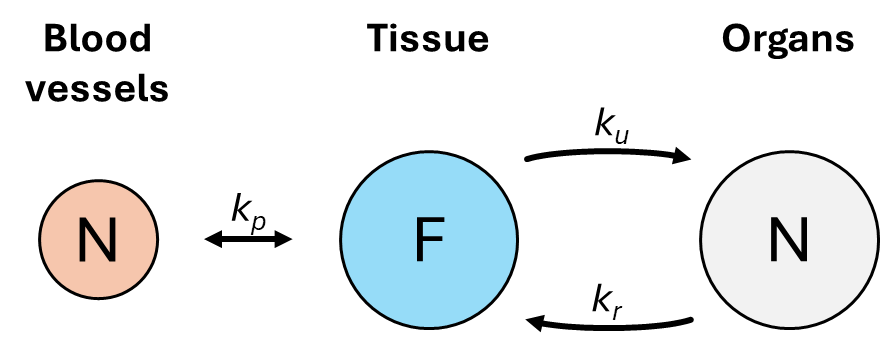
../../_images/drug_treatment_fig2.png — Fig. 2 Schematic of the constructed pharmacokinetic model.#

For the calibration of the aforementioned parameters (the drug’s decay coefficient and the transport rates between the tissue and the organs), we utilize one of the data sets published in Drexler et al. (2020).

Fig. 3 shows the drug concentrations measured in one of the mouse’s blood over time following a single 8 mg/kg bolus injection.

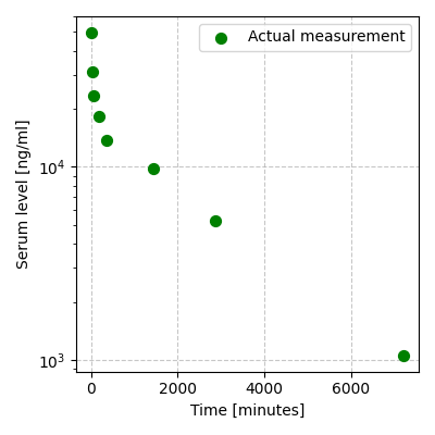
../../_images/drug_treatment_fig3.png — Fig. 3 Time course of drug concentration measured in blood. (Re-plotted from data in Drexler et al. (2020).)#

The treatment is represented by an Event object in our LattiCS model. This event will be scheduled immediately at the start of the simulation and will trigger a change in the concentration of the substrate named “drug” to a specified value (which is also a placeholder value here).

treatment_1 = lattics.Event(
        time=(0, 'sec'),
        handler=set_substrate_level,
        concentration=1.0,
        name='drug'
        )
simulation.add_event(treatment_1)

Our model is now ready to be executed and the resulting data retrieved. Consistent with the measurement data shown in Fig. 3, we will simulate a 5-day duration, using the previously set 30-second time step for the substrate. Data logs of the simulation will be stored after every 10 simulated minutes, but the data will only be written to a file upon completion (for a short simulation like this, continuous file writing could slow down the execution).

simulation.run(
        time=(5, 'day'),
        dt=(30, 'sec'),
        dt_history=(10, 'min'),
        save_mode='on_completion'
        )

After plotting the concentration profile established in the simulation space (see Fig. 4 (A)), it is clear that the model parameters require refinement, as the simulated data set deviates significantly from the real data. Although this calibration could be performed using any of the well-established parameter fitting routines, we instead employ an “eyeballing” approach here to heuristically tune the model’s parameters and gain a better understanding of their sensitivity and impact on the system dynamics.

In the simulated data, the drug concentration settles to an equilibrium value after a long period (meaning the drug is transferred from the blood vessels into the tissues). However, this equilibrium concentration is orders of magnitude lower than the initial drug concentration observed in reality, and the steady-state is reached too slowly. Let’s first modify the concentration value within the Event representing the treatment so that the resulting equilibrium concentration roughly matches the initial value of the real data set (10⁶ is an approximately good choice, see Fig. 4 (B)).

Next, we modify the rate of transfer from the blood vessel node into the tissues by increasing the passive_rate parameter stored in the blood_vessel_transport_info variable (5 × 10^-1 is an approximately good choice). Following these changes, the simulated drug concentration in the tissues will approach the initial value of the real data set (see Fig. 4 (C)), but the elimination dynamics still remain unrealistic.

In our model, the drug can leave the system due to decay, the rate of which was set during the substrate creation. Let’s modify the decay_coefficient and set a small but non-zero value (e.g., 10^-8). As a result, the trend of the simulated curve begins to resemble that of the measured data; however, the dynamics are still not perfect (see Fig. 4 (D)). In our model, decay is a first-order reaction, meaning the concentration decreases exponentially, whereas in the real data set, the elimination rate gradually slows.

Let us now set the release_rate and uptake_rate values stored in the organs_transport_info variable. We set the rate of uptake (flow from tissues to organs) greater than the rate of release (e.g., 1.0 and 5.0, respectively). Due to this change, the characteristic change in drug concentration begins to follow the trend of the real data set (see Fig. 4 (E)). Further adjustments to these parameters can quickly yield an adequate approximation.

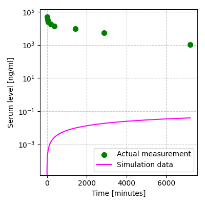
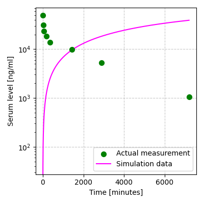
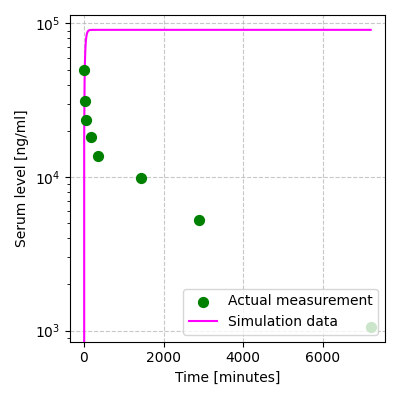
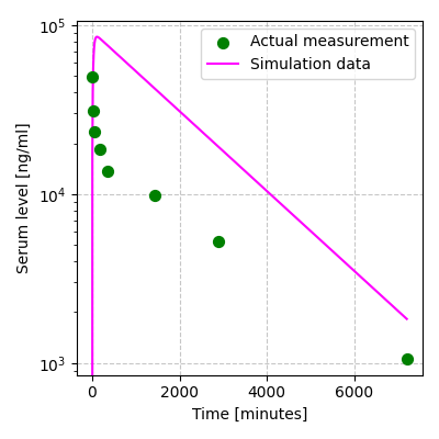
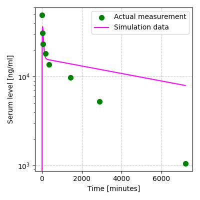
(A) — Fig. 4 Concentration profiles generated during the stepwise fine-tuning of the substrate parameters.#

(B) — Fig. 4 Concentration profiles generated during the stepwise fine-tuning of the substrate parameters.#

Tumor growth#

Next, we add the agents representing the tumor cells to the model. The changes observed in the tumor cells in the original ODE model are implemented using the following LattiCS components.

Cell proliferation. We describe cell proliferation by adding a cell cycle component to the simulation. When creating any component, we must set its update timestep (this defines how often the component can update the agents’ characteristics, in this case, whether or not the agent needs to double in that specific step). We set this to 1 hour to match the update interval of the simulation space (however, the two intervals can be configured differently).

from lattics.models import FixedIncrementCellCycleModel

cellcycle_model = FixedIncrementCellCycleModel(update_interval=(1, 'hour'))
simulation.add_model(cellcycle_model)

The doubling time can be set when the agent are added, as it may be different for each agent. (The component implements the general cell cycle model but fetches and applies its parameters individually to each agent to manage that agent’s unique state.)

Spontaneous necrosis of cells. Cells can undergo apoptosis (cell death) even independently of the drug concentration. Since the model does not account for the reasons behind this, we model this spontaneous necrosis as a random process.

from lattics.models import StochasticTransitionModel

necrosis_model = StochasticTransitionModel(
        update_interval=(1, 'hour'),
        condition=('state', 'live'),
        end_states={'state': 'necrotic', 'division_pending': False},
        rate=5e-10
)
simulation.add_model(necrosis_model)

Concentration-dependent necrosis of cells. Apoptosis in cells can also be initiated based on the level of intracellular drug concentration. As the exact mechanistic steps of the drug’s action are not detailed in the original model, we treat this process in LattiCS as a random event. According to the original model, the time-unit cell death probability increases with concentration until it hits a saturation limit, beyond which further concentration increases have no effect. The median_effective_concentration) defines the drug concentration at which the probability of cell death is exactly 50%.

toxicity_model = ConcentrationDependentToxicityModel(
        update_interval=(1, 'hour'),
        substrate_name='drug',
        max_rate=1e-3,
        median_effective_concentration=1e-5
        )
simulation.add_model(toxicity_model)

Necrotic cell washout. Cells in a``necrotic state`` are eventually cleared or otherwise disappear from the tissue. Since the model does not include the exact process of this, we also model the washout as a random process, in which the transition component marks the necrotic cells with a remove_pending label. As a result, they are deleted from the space and from the agents in the next step of the simulation.

washout_model = StochasticTransitionModel(
        update_interval=(1, 'hour'),
        condition=('state', 'necrotic'),
        end_states={'remove_pending': True},
        rate=1e-9
        )
simulation.add_model(washout_model)

References#

Drexler et al. (2020) Dániel András Drexler, Tamás Ferenci, András Füredi, Gergely Szakács, Levente Kovács, “Experimental data-driven tumor modeling for chemotherapy”, IFAC-PapersOnLine, Volume 53, Issue 2, 2020, Pages 16245-16250, ISSN 2405-8963; https://doi.org/10.1016/j.ifacol.2020.12.619

Claridge et al. (2007) Ela Claridge, Džena Hidović-Rowe, Phillipe Taniere, Tariq Ismail, “Quantifying mucosal blood volume fraction from multispectral images of the colon”, Proc. SPIE 6511, Medical Imaging 2007: Physiology, Function, and Structure from Medical Images, 65110C (29 March 2007); https://doi.org/10.1117/12.709559

Qi et al. (2008) Xiu-Ling Qi, Peter Burns, Juimiin Hong, Jeff Stainsby, Graham Wright, “Characterizing blood volume fraction (BVF) in a VX2 tumor”, Magnetic Resonance Imaging, Volume 26, Issue 2, 2008, Pages 206-214, ISSN 0730-725X; https://doi.org/10.1016/j.mri.2007.05.010

Lee et al. (2021) Benjamin J. Lee, Yahya Cheema, Shahed Bader, Gregg A. Duncan, “Shaping nanoparticle diffusion through biological barriers to drug delivery”, JCIS Open, Volume 4, 2021, 100025, ISSN 2666-934X; https://doi.org/10.1016/j.jciso.2021.100025

Schleyer et al. (2024) Genevieve Schleyer, Eann A. Patterson, and Judith M. Curran, “Label free tracking to quantify nanoparticle diffusion through biological media”, Sci Rep 14, 18822 (2024); https://doi.org/10.1038/s41598-024-69506-0

Previous topic

Next topic